Upload Tool
Microsoft, Windows, Excel, and Visual Basic are trademarks or registered trademarks of Microsoft Corporation.
Introduction
The upload tool is an Excel spreadsheet with Visual Basic macros which produces a text file in JSON format from data defined in the spreadsheet. The resulting text file can be uploaded to the service as described here.
JSON is a lightweight and human-readable data format which can easily be generated and parsed. It consists
of a dictionary of key-value pairs
where key
is a string and value
can be either a string, number, boolean, a list of values,
or another dictionary of key-value pairs. This allows for nested data structures.
Data in Excel on the other hand is stored in flat, table-like ranges, and in order to produce nested data structures we need commands which control how the
data ranges are assembled into a JSON structure. The control commands start with a keyword followed by the worksheet name followed by the address of the
upper left cell of the data range (in A1 notation) with |
as separator, for instance !ToListOfDicts|QCSetup|B20 tells the
upload tool that the data range with upper left cell B20
in worksheet QCSetup
should be transformed into a list of dictionaries.
The allowed keywords are:
- !ToDict: a dictionary - each row of the data range represents a key-value pair. The keys are taken from the first column of the data range and the values from the second. Values might also be control commands here.
- !ToList: a list - takes the values of the list from the first column of the data range. Values must not be control commands here.
- !ToListOfLists: a list of lists - each row of the data range represents a separate list of values. If at least one cell is emtpy the entire row is ignored. Values must not be control commands here.
- !ToListOfDicts: a list of dictionaries with the same set of keys - the first row of the data range is the header and contains the keys of the dictionaries. The following rows contain the corresponding values of each dictionary. If a cell in a value row is empty this key-value pair is ignored for that particular dictionary. Values might also be control commands here.
- !ToListOfRefs: a list of control commands - takes the values of the list from the first column of the data range. Only control commands !ToDict and !ToListOfDicts are allowed here, everything else will be ignored.
In order to determine the size of a data range when the upper left cell is given the upload tool follows this procedure: starting from the upper left cell, the upload tool crawls in the same row to the right until an empty cell is found. The cell immediately before that empty cell is the upper right cell and its coordinate determines the number of columns in the data range. After that the program starts to scan row-by-row the content between the upper left cell and the upper right cell until a row is found with all the cell content empty. The row immediately before that defines the lower left and lower right cells of the data range.
Please be aware that there are no safeguards implemented in the upload tool which prevent you from circular references or from creating absurdly deep nested data structures.
Description of the Worksheets
QCSetup
This is the control panel of the upload tool. It contains the button which triggers the JSON file generation, as well as the location of the
file output in cell B2 (named range FileLocation
) which you have to adapt to your installation, and the number of simulation scenarios
in cell B4 (named range nbrSims
). The outermost
dictionary of the JSON data structure has its upper left cell at B9
(named range root
) with the definition of the Reference Date followed by links to the nested data structures for YieldCurves, Instruments,
TimeSeries etc.
No worries if the locale you are using in Excel does not comply with the ISO date format or the
point as decimal separator which are mandatory in the JSON data structure:
the upload tool will take care of this. The only exception is the
par trade convention
for instrument coupons (or spreads or strikes),
for instance @par+0.001, where you really have to use the point as decimal separator independent of your locale.
YieldCurves
You can define the content of the built-in yield curves here. Since the term structures are stored as zero rates you have to provide a
daycount convention and a compounding method, as well as an interpolation method for dates between grid points. For the upload you can either
specify zero rates or discount factors (using a list of lists data range with key ZeroRates
or DiscountFactors
, respectively).
The data ranges with the term structures contain tenors in the first column and the zero rates (or discount factors) in the second.
Those yield curves for which you do not specify data here, will not be affected when you upload the JSON file to the service.
TimeSeries
You can specify the content of the built-in time series here - either by referring with key Data
to a list of lists data range containing
the historical observations or by a default value with key DefaultValue
which is used whenever a historical reset/fixing is needed.
Instrument Types
The following worksheets are for creating instruments of different type. Please refer to the example instruments for valid key-value pair settings, and to this page for an explanation of the fields.
Portfolios
You can define portfolios and their content here - either by referring with key AliasList
to a list data range containing
the aliases of the instruments in the portfolio or by a Regular Expression search pattern with key SearchPattern
.
Scenarios
You can define Stress Scenarios here. The yield curves and FX rates to be shifted are contained in
list of dicts data ranges which are referred to by keys YieldCurves
and FXRefIndices
, respectively. Both keys are mandatory,
that is you have to provide an empty list of dicts data range even if you do not want to shift any FX rates or yield curves at all.
For each yield curve or FX rate to be shifted you have to specify the spread type described here. While
for FX rates it is sufficient to define the spread by a single number, you have to specify an interpolation type and a term structure of
spreads for yield curves. This is achieved by referring to a dict data range for each yield curve to be shifted under key Spread
.
Please note that in this dictionary the index of the
grid point where the spread is to be applied has to be given as string: 0
is the first grid point, -1
the last one.
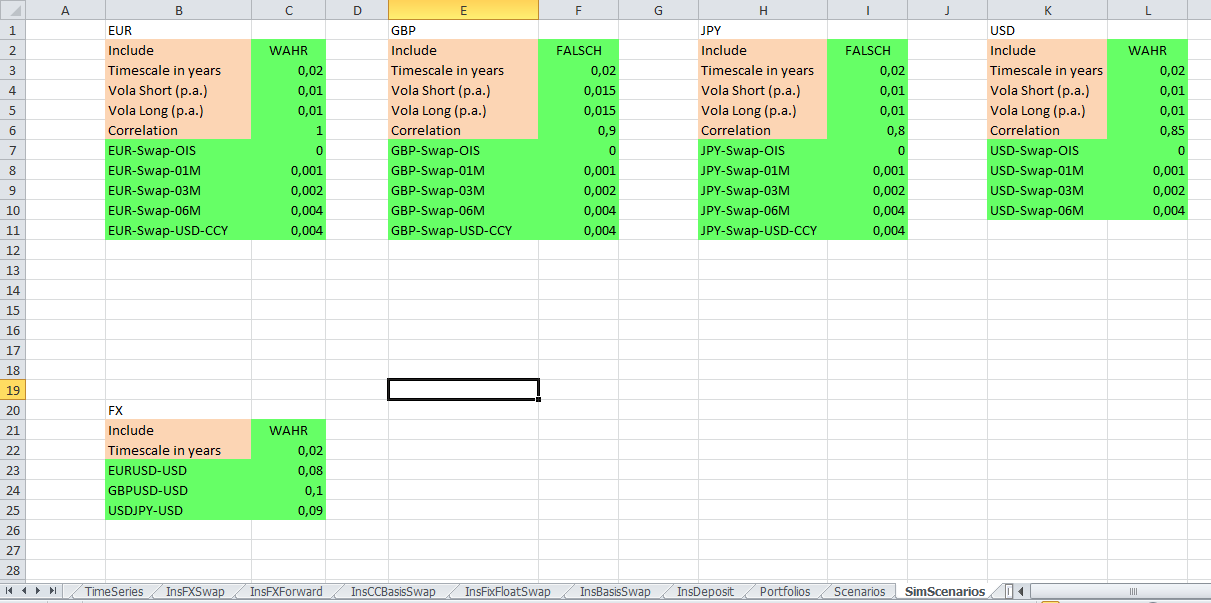
SimScenarios
This worksheet shows how you can produce Simulation Scenarios for the service with a Monte-Carlo engine. Please keep in mind that this is an example with highly simplifying assumptions for illustrative purposes only.
For the scenario generation for yield curves we assume three driving factors per currency, represented by the three Brownian motions dWshort for the short end of the curve, dWlong for the long end, and dWspread driving the spreads within that currency. While dWlong and dWshort are correlated with given correlation coefficient ρ, dWspread is uncorrelated to the other two Brownian motions. For each yield curve i within one currency we then assume the spread on the short end (applied to the first grid point) dSishort and the spread on the long end (applied to the last grid point) of the yield curve dSilong to be given by
dSishort = σshort dWshort + σispread dWspread
dSilong = σlong dWlong + σispread dWspread
with
E[dWshortdWlong] = ρdt, E[dWshortdWspread] = E[dWlongdWspread] = 0
E[dW2short] = E[dW2long] = E[dW2spread] = dt
The normal yield volatilities for the short and long end, σshort and σlong,
the normal spread volatilities for each curve σispread, and the correlation coefficient are taken
from the spreadsheet for each currency. The field Timescale in years
defines the liquidation horizon of the simulation:
for a horizon of five business days we have 5/250 = 0.02. You can switch on and off the scenario generation for each currency with the
field Include
.
If you switch on FX scenario generation, an uncorrelated geometric Brownian motion is assumed to drive the exchange rate for each currency pair. The corresponding log-normal volatilities are taken from the spreadsheet.
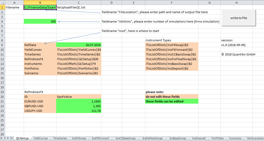
QCSetupin the upload tool
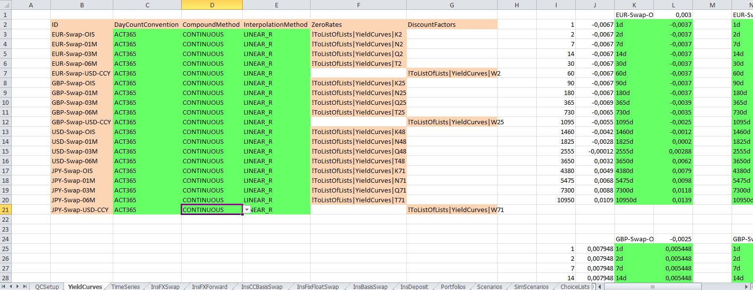
YieldCurvesin the upload tool
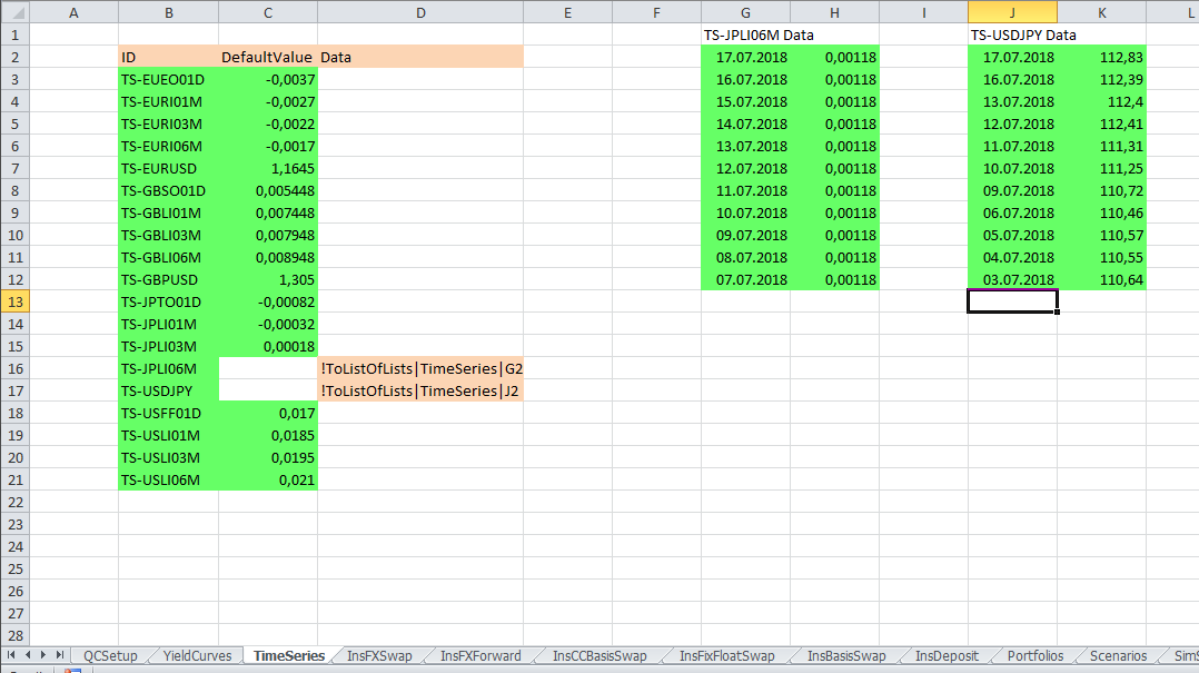
TimeSeriesin the upload tool
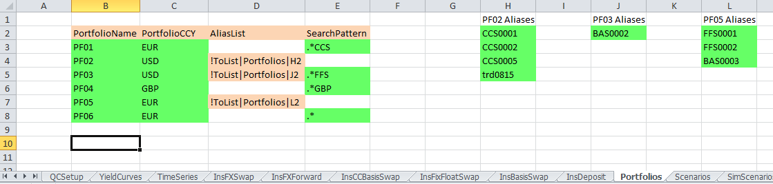
Portfoliosin the upload tool
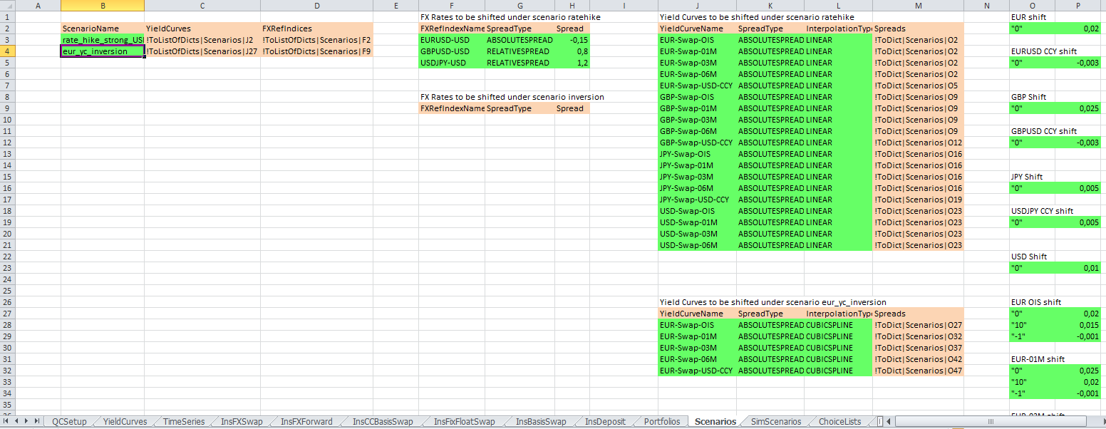
Scenariosin the upload tool
SimScenariosin the upload tool